// feature selection

Filter Methods

There are various kinds of statistics that are mentioned in the section on Inferential Statistics. Those statistical tests are used under filter methods to find the independent feature’s relation with the dependent variable, and based on the scores, it is decided if the features are to be kept or discarded.

Process of Filter Methods

To avoid confusion, you must remember that this feature selection process is free of the machine learning algorithm, and individual statistical scores of features are used to reduce the features.

Filter Methods are a particular pre-processing step performed before the modeling is done (as other feature selection methods, such as Embedded and Lasso, are not really data preparation, as features are reduced during the modeling process; however, they are included under the section of data preparation, as feature reduction falls under data preparation, and they, after all, do help in reducing the dimensionality of the dataset).

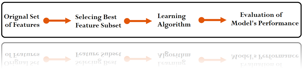
Filter Methods are useful, as they are simple to understand and give us insights about the data; however, they cannot be called the best technique to optimize the features for better generalization (prediction, classification, etc.). The process to reduce dimensions using a Filter Method is simple: we select our features, we perform various filtering methods on each of these features depending upon the type of feature (character/numerical) and the relation it shares with the dependent variable (linear/non-linear), and after performing the filtering methods, the significant features are selected to form a subset of features which is used in the model, and after assessing the model’s performance, tweaks can be made in selecting the features to come up with the best subset of features that provides the best performance.

Types of Filter Methods

Pearson’s Correlation

Pearson’s Correlation has been explained in detail in the blog on Correlation Coefficients. Pearson’s Correlation can be used for reducing the numerical features, as correlation can be tested between the various numerical independent variables in the dataset and the numerical dependent variable (Y-Variable / Outcome variable). If the correlation is high enough, then the feature is selected (close to -1 or 1), and if the correlation coefficient is low (close to 0), then such a feature can be dropped. Thus, by measuring the linear dependency of the X and Y variables, we can decide whether we want to keep a particular feature or not. However, Pearson’s correlation suffers from a major drawback: it cannot be used to reduce those features which share a non-linear relationship with the dependent variable, so for a symmetric non-linear relationship (for example a U-shaped one), the positive and negative deviations cancel out and the correlation can come out close to 0, thus providing misleading results. Therefore, Pearson’s correlation will not help in reducing the number of features under such scenarios, and for such scenarios, another kind of correlation, such as Mutual Information and Maximal Information Coefficient (MIC), should be used, which is a more sophisticated filtering method. Still, one should bear in mind that if the relation is linear, Pearson’s Correlation has an edge over other correlations, as it is fast (which is important when dealing with voluminous datasets), and the correlation coefficient range is between -1 and 1 (which some others don’t have), and this negative range provides us with extra information about whether the relationship is negative or not.

Mutual Information and Maximal Information Coefficient (MIC)

As explained above, there are certain limitations of Pearson’s Correlation, and this limitation can be resolved by using a more sophisticated kind of correlation, which is Mutual Information Correlation, which rigorously quantifies (in a dimensionless quantity, in units known as “bits”) how much information the values of one variable reveal about the values of another. The outcome of such a coefficient ranges from 0 to N, where 0 (unlike Pearson’s Correlation with non-linear relationships) actually means that there is zero mutual information between two variables, meaning that the two variables are independent.

The range of the outcome leads to a problem, as the range is not fixed and the values are also not normalized (unlike Pearson’s Correlation, where the range of the coefficient is fixed from -1 to 1 and the values are normalized in the sense that coefficients found from different variables can be compared), making it difficult to compare different Mutual Information values. This is where another type of correlation can be used, the Maximal Information Coefficient, where the mutual information score is converted into a metric that can lie in a range between 0 and 1; however, as discussed before, this range also provides only half the information, as negative relations are not explained, but it can still be used for variables sharing a non-linear relationship.

ANOVA

ANOVA has been discussed in the section on F Tests, where the use of ANOVA to find the relationship between variables has been discussed. It is recommended to first go through that section. ANOVA can be used to find whether the numerical dependent and categorical independent variables share any relationship, where the independent variable has two or more groups (levels). Thus, it runs a statistical test to find whether the means of several groups are equal or not. However, it may suffer from a drawback where ANOVA may indicate that variables have no relationship, but it can be possible that one of the groups (levels) was actually related to the dependent variable, but due to the lack of dependency of the other groups with the dependent variable, the outcome from the ANOVA made us drop the feature, causing us a loss of information. This is why, under such circumstances, the categorical variables are encoded and ‘decomposed into numerical variables’ so that these variables can then be used for reducing the features by methods which require the features to be numerical.

Chi-Square

This statistical tool has also been discussed in Chi-Square, and it is recommended to go through it first. Chi-square can be used when the dependent and the independent variables are both categorical. A typical example of this is when dealing with classification problems where the dependent variable has categories. If the independent variables are also categorical, then a chi-square test can be run, and the features that don’t share a relationship with the output variable (Y Variable / Dependent variable) can be dropped. However, if there are a lot of categorical variables having numerous categories, it is better to encode the categorical variables and use more sophisticated feature reduction methods that require the features to be numerical. Also, running chi-square for multiple categorical variables can be time-consuming, and other faster, more sophisticated methods may be deployed for the reduction of dimensionality.

LDA (Linear Discriminant Analysis)

LDA is used to reduce the number of features, as it preserves the interclass separation present in the original feature vector by finding a linear combination of features that characterizes or separates two or more classes (or levels) of a categorical variable. A PCA (Feature Extraction method) can be used for reducing the number of variables, but it will only end up giving us the list of our features with their leading eigenvalue, indicating which features affected our data the most. However, if we have some prior information or intuition that the data points of the dataset have different classes and want to preserve these classes while reducing the number of features, LDA can be used, as it will let us know the features/combination of features that are affecting class separation.

Using Models

A machine learning model can also be built to find the important variables. For example, we can create a linear regression model which uses standardized regression coefficients for prediction (which is somewhat equivalent to Pearson’s correlation) and can use all our features, and from the output we can get information about the effect of features on the dependent variable and select the top significant features. A similar practice can be done for classification problems by using logistic regression, and if the variables are non-linear, then tree-based models can be used. However, this method is not recommended, as it can easily lead to the problem of overfitting, where, for example, the top 5 important variables are related to the dependent variable but hold essentially the same information, causing the model to overfit.

Filter Methods are among the easiest to understand methods that can be used to reduce the number of features in the data. The main drawback of these methods is that they are essentially univariate selection processes, making the process of feature reduction very slow. Also, even though they help us by providing the variables that are important for our model by checking the relationship they share with the dependent variable, they are unable to remove redundancy (i.e. check whether these important variables hold the same information, in other words check for multicollinearity). Thus we require selecting features from among these related features so that we can decrease multicollinearity, providing our model with the best accuracy without causing it to overfit. To select the best feature among a subset of strongly correlated features, we use other feature selection methods, such as Wrapper Methods (where Stepwise Regression and other techniques are used) or Embedded Methods (where Linear Models and Regularization techniques are used).