// shared: regression & classification

Decision Trees

A Decision Tree is “a decision support tool that uses a tree-like graph or model of decisions and their possible consequences”. In this article, we explore algorithms based on decision trees used for either prediction or classification. Decision Trees can be tricky to apply, as it is sometimes confusing to understand when to use them. Generally, decision trees can be used when the data is of fairly poor quality. Tests such as the Hosmer-Lemeshow test can be undertaken to see if the data is fit for logistic regression or not. Also, when the data or the situation is very complex and difficult to explain to a client, decision trees can be used, as they provide level-by-level control over the classification process, whereas logistic regression works like a black box where we feed in the data and it produces the output. Also, decision trees aren't affected by outliers or missing values, and don't require the transformation of data, as they try all possible thresholds and all possible features and are thus very robust in this sense.

Regression Trees v/s Classification Trees

Decision Trees can be of two types: Regression Trees and Classification Trees. Regression Trees are used when the dependent variable is a continuous variable and we need to predict its value, while Classification Trees can be used as a proxy for logistic regression. Here, Classification Trees, like logistic regression, can be used to find whether a combination of x variables will result in Y=1 or not. Procedures such as CART, CHAID, and C4.5 can build classification trees. CART and CHAID handle both two-category and multi-category targets, while C4.5 is commonly used when the target has more than two categories.

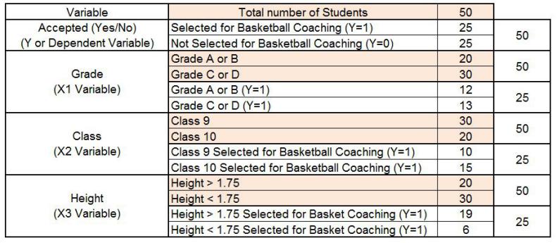
An example to understand classification trees can be a dataset where the dependent variable is whether a grade 9 student is selected for a basketball coaching camp or not. For the independent variables, we have the height, weight, and marks of the student. The classification tree now has to decide, based on these three variables, whether the students will be selected for the basketball coaching camp or not. The classification tree first classifies students on a criterion that acts as the single biggest contributor in deciding whether the students will be selected or not. Here the homogeneity of the data is considered. For example, if the decision tree finds that 95% of students who are taller than 1.73 meters are selected for the camp, then this makes the data 95% pure. Different measures (such as Chi-Square, Gini Index, Entropy, etc.) are used to make this decision as ‘pure’ as possible. This binary splitting of the data is the essence of how a classification tree works.

On the other hand, Regression Trees are typically built using CART (decision trees do not assume a linear relationship and can capture non-linear ones). CART (which does binary recursive partitioning) is used to keep the splits ‘pure’, wherein, in each iteration of the regression tree algorithm (for example, Reduction in Variance), for all of the independent variables we find the best cut-off point ‘s’ such that if we divide the data into two, the mean squared error of the sample below ‘s’ plus the mean squared error of the sample above ‘s’ is minimized. Once this is done for all of the independent variables, the variable that gave the best (lowest) mean squared error is selected. In other words, to find the first split, each independent variable is split at several points and the error is found (the difference between predicted and actual value), and the split point with the lowest error is chosen to split the data. This process is recursively continued until any further step gives too little gain in the MSE.

One must note that classification trees are commonly referred to as Decision Trees, as Decision Trees are most commonly used for classification purposes only; for this reason, this article will mainly discuss classification trees, with occasional reference to regression trees.

Advantages of Decision Trees

Decision Trees provide high accuracy and require very little preprocessing of data, such as outlier capping, missing value treatment, or variable transformation. Also, they can work even if the dependent and independent variables are not linearly related, i.e. they can capture non-linear relationships. Decision Trees require less data than a regression model and are easy to understand, along with being highly intuitive. Tree-based models can be very easily visualized with clear-cut demarcation, allowing people with no background in statistics to understand the process easily. Decision Trees can also be used for data cleaning, data exploration, and variable selection and creation. Decision Trees can work with both continuous and categorical variables.

Greedy Algorithm

The Decision Tree follows a Greedy algorithm. For example, if the chosen algorithm is Chi-Square, then at each step the greedy algorithm performs a Chi-Square test and checks whether the independent variable is associated with the dependent variable. Thus, it considers all the variables and selects the one that provides the most ‘pure’ split. It finds the best solution at each stage, and once found, repeats the process to find the best optimal solution for the next stage.

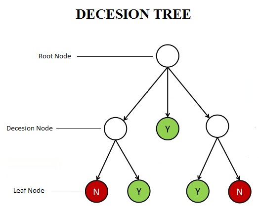
Important Terms

Decision Node: Any node that gets split is known as the decision node.

Root Node: This is the topmost decision node, and represents the entire sample, which gets further divided.

Leaf Node: Also known as the terminal node, this is a node that does not split further.

Splitting: The process of dividing a node is known as splitting.

Pruning: This is the opposite of splitting; here we remove sub-nodes of a decision node.

Methods of Creating Decision Trees

As occasionally mentioned above, there are multiple methods through which decision trees can be created. Each of these methods uses certain algorithms as decision criteria to create and increase the homogeneity of the sub-nodes.

There are many well-known methods, such as:

ID3: The Iterative Dichotomiser 3 is the core algorithm for building decision trees and uses a top-down approach (splitting). It uses Entropy (Shannon Entropy) to construct classification decision trees. As ID3 uses a top-down approach, it suffers from the problem of overfitting.

C4.5: This method is the successor of ID3. It is used for building classification trees, including when the dependent variable has more than two categories. It was a major improvement over ID3, as it could handle both continuous and categorical dependent and independent variables. It was also able to solve the overfitting problem (discussed below) by using a bottom-up approach (pruning).

C5.0: Some improvements were made over C4.5. These were better speed and memory usage, and, most importantly, the incorporation of boosting, an ensemble learning algorithm.

CART: Among the most common, it is a non-parametric decision tree learning algorithm, with its full form being Classification and Regression Trees. It is similar to C4.5, but uses the Gini Impurity algorithm for classification, where the aim is to make each node as ‘pure’ as possible.

CHAID: The Chi-Square Automatic Interaction Detector actually predates ID3 by 6 years, and can be used for regression and classification trees; it is a non-parametric approach, as it uses Chi-Square as the metric to build classification decision trees.

Other algorithms used in decision trees include MARS, QUEST, CRUISE, etc.

Algorithms of Decision Trees

The numerous decision tree algorithms mentioned above use various metrics to decide how to split the nodes. The most common criteria/metrics for Classification Trees are:

Gini Index, Entropy, Chi-Square (for Classification Trees), Reduction in Variance (for Regression Trees), and ANOVA.

To understand how these methods work, we will consider a dataset, briefly introduced earlier, where the dependent variable is whether a student was selected for the school basketball coaching camp or not. For the independent variables, we will take two categorical variables and one continuous variable. The two categorical variables here will be Academic Grade (A or B, and C or D) and Class of the student (9th and 10th grade), with the continuous variable being Height.

Metrics for Classification Trees

Gini Index

This method is used in CART and only performs binary splits. The formula for calculating the Gini Index sums the squared probability p_i of an item belonging to the chosen label ‘i’, subtracted from 1. It reaches its minimum (zero) when all cases in the node fall into a single target category.

We find that out of a total of 50 students, half of them were selected for the coaching camp. For calculating the Gini Index, we have to find the proportions of these values.

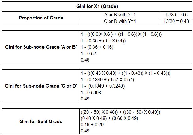
Now we can find the weighted Gini for split X1 (Grade) by calculating the Gini for the sub-nodes ‘A or B’ and ‘C or D’.

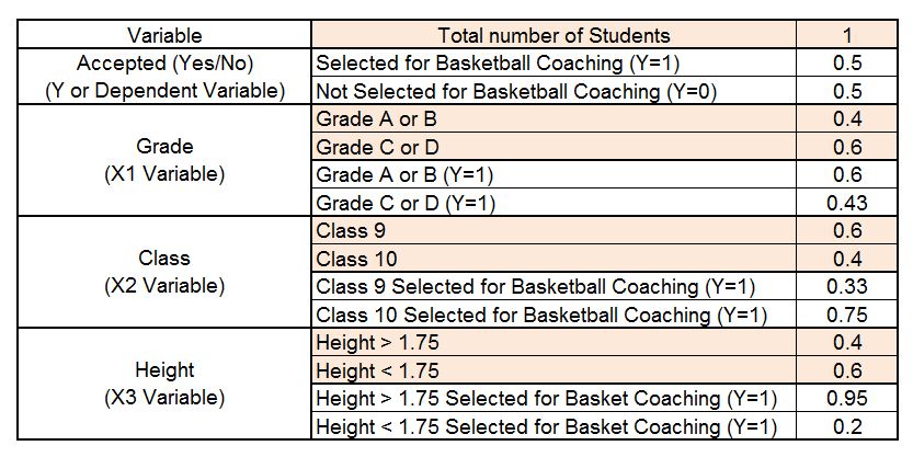
We can similarly do the same for X2, which here is Class, and find the Gini for splitting on Class.

For X3, Height, which is a continuous variable, the statistical software in the backend splits the variable into height > x and height < x, and finds the Gini value; whichever value of x provides the minimum Gini value is used to calculate the Gini for splitting this continuous variable. In our example, we find that the value of x equal to 1.75 provides the minimum value, compared to other values of height, say 1.80 or 1.60. We find that the Gini for the height split comes out to be 0.23.

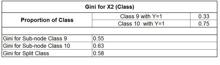
Now we compare the values of Gini and find that the minimum Gini is provided by Height (0.23); thus this variable will be the root node that splits the data into two homogeneous, ‘purer’ sets. The second-minimum Gini value is found for the Grade variable, and the maximum Gini value is found for Class. Thus, the data will first split by Height, as it plays the major role in deciding whether a student will be selected for the basketball coaching camp or not.

Entropy

Entropy is an algorithm used by ID3, where it measures the amount of uncertainty in the data to decide which variable will be used to split. Here we find the variable that needs the least information to describe itself, and this is measured by entropy. If the data is completely homogeneous, the value of entropy will be 0, while if the variable is completely disorganized and equally divided, the value of entropy will be 1.

The formula for Entropy is:

H = −p·log₂p − q·log₂q

with p and q being the probability of Y=1 and Y=0 in each variable.

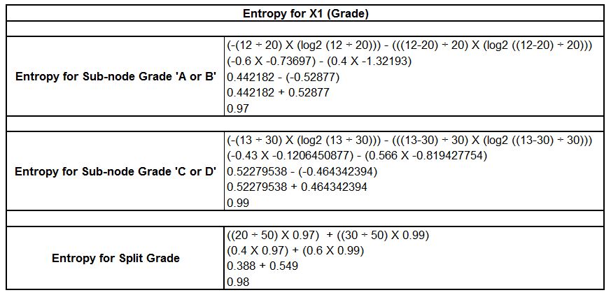
(Below we use the basketball coaching dataset.) If we find the entropy of the parent node (the parent node is the node which is sub-divided; here the dependent variable is the parent node), it comes out to be 1, as in our example it is impure, with equally divided categories (25 students selected and 25 students not selected). The calculation is shown below:

= −(25/50) × log₂(25/50) − (25/50) × log₂(25/50)
= −(0.5 × −1) − (0.5 × −1)
= −(−0.5) − (−0.5)
= 1

Thus, it is a very impure node. We now look for the root node. We calculate the entropy for different categories of the independent variable, and find the entropy for each independent variable in the process. First, let's calculate the entropy for the X1 variable, which is Grade.

We can similarly do the same for X2 and X3, which here are Class and Height, and find the entropy for splitting on Class and Height.

Note: As Height is a continuous variable, statistical software uses entropy for every single value and splits on the value that provides the minimum entropy. Equal-size bins can also be used to make the process less time-consuming.

On comparing the values of entropy, it seems that the split on Height should once again be done first, as its entropy is the lowest, meaning it provides the purest node.

Chi-Square

As mentioned above, Chi-Square is used in CHAID. Here, the decision tree algorithm performs a chi-square test and finds the chi-square values. The higher the chi-square value, the more significant the variable is in determining the split. Detailed calculation of chi-square will not be discussed in this article, as it has already been covered in the article on Chi-Square, and it is advised to go through that article if you want to understand how the calculation is done to find the chi-square value.

Metrics for Regression Trees

Reduction in Variance

When the dependent variable is continuous, we use Reduction in Variance, where the variable selected for the split is the one that provides the lowest variance (refer to Measures of Variability to know more about how variance works).

The formula for variance is:

∑(x − x̄)² ÷ n

However, when the variable is categorical, it can get a bit more complicated. Below are the calculations for finding the variance for the two categorical variables in our example, X1 and X2 (Grade and Class). Here x is the value and x̄ is the mean of the variable, while n is the total number of records. We have assigned 1 for students who got selected (Y=1) and 0 for students who got rejected (Y=0); we will not use these 1s and 0s themselves to calculate the mean and deviation, but rather as the values being averaged.

For example, let's calculate the mean and variance for the root node. Here we have 25 1s (Y=1) and 25 0s (Y=0). We calculate the mean as ((25 × 1) + (25 × 0)) ÷ 50, which comes out to be 0.5. We can now use the formula for variance; here our x̄ will be 0.5, while x will be 1 or 0. We have 50 entries, so the formula can be written more compactly as (1 − 0.5)² × 25 + (0 − 0.5)² × 25, all divided by 50.

We use this formula to find the mean and variance for each variable. Below is the calculation to find the variance of the X1 (Grade) variable.

We can use the same formula to find the variance for splitting on Class.

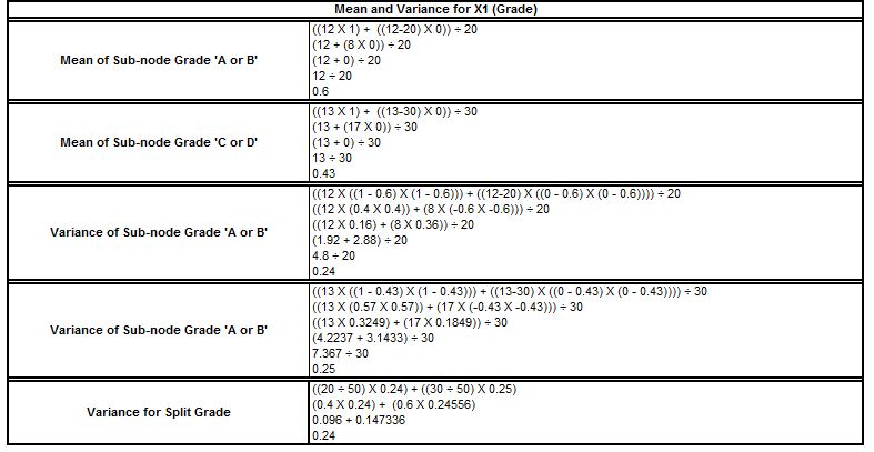
We find that the results are similar to entropy, with Grade being the least important variable, as its variance (0.24) is higher than the other categorical variable, Class, which has a variance of 0.21. The variance of the numerical variable follows similar steps, and the variable that provides the minimum variance is considered for the split.

ANOVA

Analysis of Variance can also be used for splitting, where we check whether the means of two groups are similar to each other or not. Here, the split happens for all variables, and ANOVA is run for all the subgroups of the variables; the variable that provides the highest F value is used to split the sample. To learn more about how ANOVA works, refer to the section on F-Tests.

Parameters of Decision Trees

One of the major drawbacks of decision trees is that they are extremely vulnerable to overfitting and can become complex very quickly. In the case of numeric independent variables, a tree can get so complex that it creates a split for each value of the numerical independent variable, thus making a leaf for each observation in the data. To solve this problem, decision trees come with a number of parameters that can be tweaked/tuned to control the complexity of the tree and prevent overfitting (these hyperparameters can be found using packages such as GridSearchCV in Python, and Caret or expand.grid in R). Also, a decision tree is a non-parametric method that can work effectively with less data compared to other modeling algorithms; however, there is one major issue with using decision trees: they show high bias and underfit in some regions of the data, while showing high variance and overfitting in other parts. This problem is addressed using methods such as K-Fold cross-validation along with ensemble methods such as Bootstrap, Gradient Boosted Trees, Random Forest, etc. These are explored in Model Validation and Ensemble Methods. Here, we take different subsets of the data to build multiple models, so that the high variance and bias present in some of the datasets can cancel each other out.

Because of the problem of complexity (overfitting) and variation in bias-variance across different samples, we often combine both of these aspects to perform a cross-validated hyperparameter search to find the right parameters that give us optimum complexity, and to use the right amount of subsetting to address the bias-variance fluctuation found in different subsets of the data (this has been explored in the application section).

In this section, we discuss the various parameters available for controlling the complexity of decision trees. The parameters can be divided into two types: parameters related to the size of the tree, used to control complexity, and parameters related to pruning, which takes a bottom-up approach to building a decision tree.

Parameters Related to the Size of the Tree

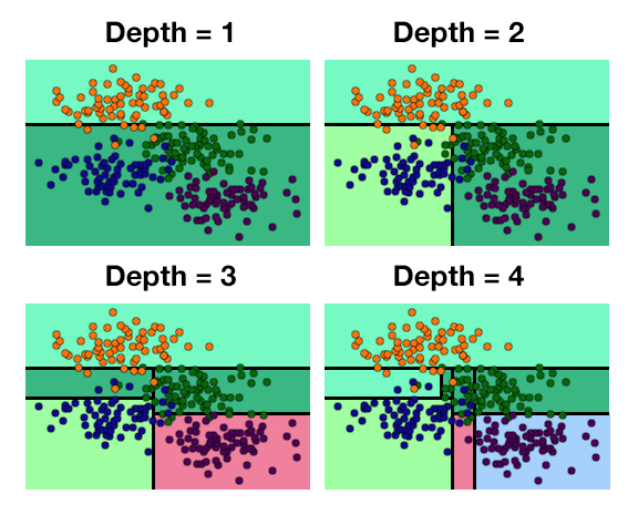
Maximum Depth

Among the easiest parameters to understand is Maximum Depth, an important parameter for tuning trees and tree-based models. It is the length of the longest path from the root node to a leaf node, or the depth of the layer of leaves. We often provide a value, maximum number, or depth limit to the decision tree model to limit further splitting of nodes, so that when the specified depth is reached, the tree stops splitting.

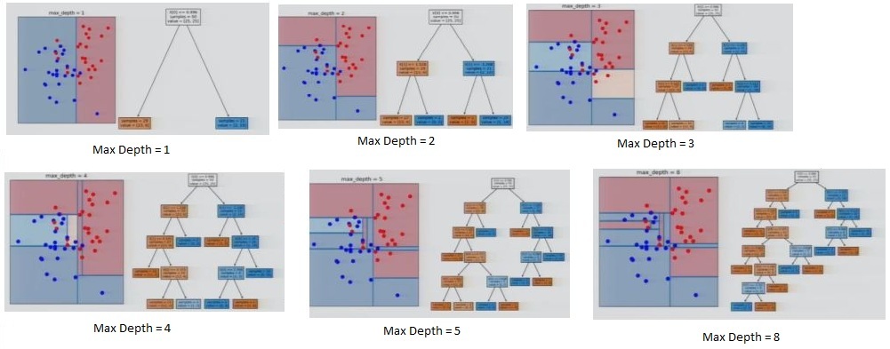
In the example above, we have two features, one on the x-axis and the other on the y-axis. Here, the tree finds that the first best split can be done on the x-axis, i.e. by splitting the variable on the x-axis and finding the value that provides the best result (the value that provides the minimum entropy or Gini, depending on which algorithm the decision tree is using). For max depth = 1, it splits the data and classifies the data points on one side as 0 (the background colour), even though some of the actual points on that side are not 0. This shallow depth makes the model too generalized and causes it to underfit. However, if the tree keeps going and recursively partitions the data, it finds further ways to split the data, creating more and more branches and further splitting the space. By the time it reaches the maximum depth, it has all pure leaves; however, this leads to overfitting, as the decision tree becomes very complex and will yield poor results on test data or unseen new data. Thus, we might set the maximum depth to 5, for example, to obtain a moderately complex and accurate decision tree model.

Minimum Split Size

This is another parameter through which we define the minimum number of observations required to allow a node to split further. This can control both overfitting and underfitting. A very low value for Minimum Split Size will lead to overfitting, with a small number of observations being considered for further splitting; however, an extremely large value will lead to underfitting, as a good number of observations that could provide useful insights upon being split won't be split.

Minimum Leaf Size

Here we provide a value that decides the minimum number of observations a terminal node must have. It is useful for imbalanced classes; for example, if we define the minimum split size at 99 and have a node with 100 observations, it can be split, but on splitting we might find that the child nodes have 99 observations in one node and just one observation in the other. We have discussed, in ANOVA and other basic statistical concepts, that each category of a variable should have a minimum number of observations to be considered for any statistical test. Similarly, here we define the minimum leaf size, which is generally around 10% of the minimum split size.

Maximum Number of Variables

We can limit the maximum number of variables a decision tree model will use, with a very low number of features causing underfitting and a very large number of features causing overfitting. Also, these features are selected randomly, so if there is a set of variables you consider very important and want to include in the decision tree, this parameter is not recommended for that purpose. Generally, around 50% of features should be considered, so if there are 100 features, the number of variables used can vary anywhere between 40 and 60, depending on the data at hand.

Maximum Impurity

In the Maximum Depth section, we saw how a low depth value caused some points to be misclassified within a region. We can similarly limit the number of misclassified points allowed within a region before splitting is stopped.

Parameters Related to Pruning

Pruning is somewhat software-specific. In R, single-tree pruning is implemented in the rpart package (via its complexity parameter, cp), and Python's sklearn also supports it through cost-complexity pruning (the ccp_alpha parameter). A Python user could also argue that, as far as predictions are concerned, we can use ensemble methods such as Random Forests, where there is no need to prune the decision tree to control overfitting. However, if we want a very simple and interpretable model, pruning a decision tree is a good idea. As briefly discussed earlier, pruning takes a bottom-up approach to building decision trees, so if we are using a top-down approach, a split that gives a negative result initially won't be considered, even though it might have led to a gain in accuracy further down the line, where the initial loss would have been tolerable (similar to what happens in Backward Elimination under Feature Selection). Pruning, however, considers overall gains and losses when deciding which nodes to split. Thus, pruning can be useful for increasing the effectiveness of the model.

Ensemble Methods of Decision Trees

Ensemble methods have been discussed in their respective section; however, to give some idea, Decision Trees can be used within Ensemble Methods, which address the bias-variance problem. When it comes to Decision Trees, the most commonly used ensemble methods are Boosting (particularly Standard Gradient Boosting and Extreme Gradient Boosting, aka XGBoost) and Bootstrap Aggregating, aka Bagging (particularly a form of Bagging known as Random Forest). To learn more about them, see Ensemble Methods.

Decision Trees are among the most powerful tools that can be used for Regression and Classification Problems. They are easy to create and understand. However, there are many methods through which Decision Trees can be created, and in this article we explored a number of them. They are, in some sense, the opposite of linear models, as they can be highly non-linear and can get very complex. However, mastering decision trees can give us insights about the data that even some other modeling algorithms can't.

Decision Trees are among the most popular, powerful, and successful learning algorithms for data modeling. Unlike other learning algorithms, they give the user better control over the whole process. This is done by allowing the user to choose from a number of algorithms, hyperparameters, etc. The whole process can also be made visual, which helps give the user a better idea of how the algorithm is working. Also, decision trees can be used for both Regression and Classification Problems.