// application · python

Regression Problems in Python

In the Theory Section of Regression Problems, a number of regression algorithms have been explored. In this blog, we will create models using those algorithms to predict the price of houses, using the following methods/algorithms:

• Linear Regression
• Regularized Linear Regression
• Decision Tree Regressor
• KNN
• Bagging Regressor (Ensemble)
• Random Forest Regressor (Ensemble)
• AdaBoosting Regressor (Ensemble)
• Gradient Boosting Regressor (Ensemble)
• XgBoost Regressor (Ensemble)
• Stacking (Ensemble)

We also perform tuning of the hyperparameters, which is done to improve the accuracy of our model and save it from overfitting. There are mainly three ways to tune these parameters: Grid Search, Random Search and Bayesian Optimization. In this blog, we will tune our parameters using the first two methods and see how the accuracy score is affected.

It is important to understand the difference between Grid Search and Random Search. In Random Search, when dealing with continuous parameters, it is important to specify a continuous distribution of plausible parameters to take full advantage of the randomization - increasing n_iter will always lead to a finer search. For each parameter, we give a range of plausible hyperparameter values; unlike GridSearchCV, not all parameter values are tried out, but rather a fixed number of parameter settings is sampled from the specified distributions. The number of parameter settings to be tried is declared through n_iter.

GridSearchCV means Grid Search Cross-Validation, wherein the program runs grid search with cross-validation. In grid search cross-validation, all combinations of parameters are searched to find the best model. The cross-validation in the code follows a k-fold cross-validation process, where the dataset is divided into train, validation and test sets. After finding the best parameter values using Grid Search, we predict on the test dataset, i.e. a kind of unseen dataset. Cross-validation helps avoid overfitting of the model. Refer to Model Validation Techniques under the Theory Section for a better understanding of the concept; hyperparameter tuning with cross-validation is discussed in Model Validation in Python under the Application Section.

In this blog, we will perform Grid Search and Random Search without explicitly mentioning the number of folds required for cross-validation. By default, Grid Search and Random Search perform a minimum of three-fold cross-validation when tuning parameters.

Importing Libraries and Preparing Dataset

Before using the dataset to create regression models, we need to import the necessary libraries and prepare the dataset.

Importing Libraries

We begin by importing the libraries that will be used throughout this blog: numpy and pandas for data handling, matplotlib for plotting, and a number of utilities from scikit-learn and scipy that we will need for model building, prediction, and hyperparameter tuning.

import numpy as np
import pandas as pd
import matplotlib.pyplot as plt
%matplotlib inline

from sklearn.model_selection import train_test_split

from sklearn import metrics

We also import the libraries required for Grid Search and Random Search hyperparameter tuning.

from sklearn.model_selection import GridSearchCV
from sklearn.model_selection import RandomizedSearchCV
from scipy.stats import uniform
from scipy.stats import randint as sp_randint

Importing Dataset

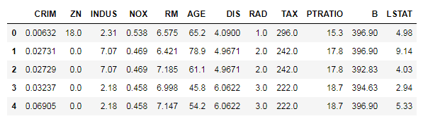
We will be using the Boston housing dataset, which is available within scikit-learn. We load it and assemble it into a DataFrame, adding the target variable (median house value) as a Price column.

from sklearn.datasets import load_boston
BostonData = load_boston()
BosData = pd.DataFrame(BostonData.data)
BosData.columns = BostonData.feature_names
BosData['Price']=BostonData.target
BosData.head()

Show full table ▾

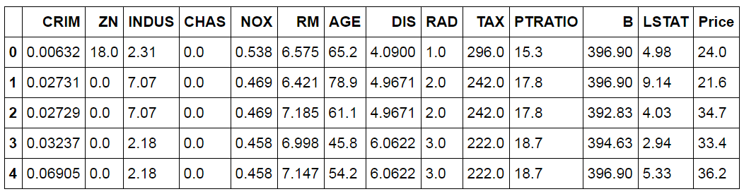
Checking for Skewness

Before modeling, it is useful to check the distribution of the dependent variable. We plot a histogram of Price.

BosData.hist(column='Price',figsize=(8,8))

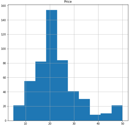
The distribution seems to be skewed. For more certainty, we use the .skew() command to measure the exact skewness.

BosData['Price'].skew()

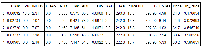
As the data is positively skewed, we will perform a transformation to reduce this skewness. We perform a log transformation on the dependent variable.

BosData['ln_Price'] = np.log(BosData['Price'])
BosData.head()

Show full table ▾

A histogram can be created to check the distribution of the log-transformed dependent variable.

BosData.hist(column='ln_Price',figsize=(8,8))

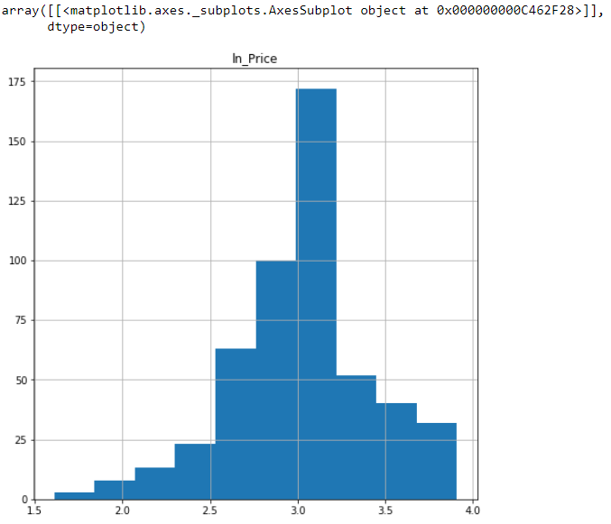
We now check for the measure of skewness in the ln_Price variable.

BosData['ln_Price'].skew()

We decide to proceed with the log-transformed variable, as it reduces the skewness of the dependent variable.

Train and Test Split

We split the dataset into a Train and a Test set, using ln_Price as the target variable.

X = BosData[['CRIM', 'ZN', 'INDUS', 'CHAS', 'NOX', 'RM', 'AGE', 'DIS', 'RAD', 'TAX','PTRATIO', 'B', 'LSTAT']]
Y = BosData['ln_Price']
X_train,X_test,Y_train,Y_test=train_test_split(X,Y,test_size=0.3,random_state=123)

The Process of Creating Regression Models

The general process we follow for creating each regression model in this blog is as follows:

• Import the required package(s) for the algorithm.
• Fit the model on the Train dataset.
• Predict on the Test dataset.
• Compute the accuracy score.

Linear Regression

To understand how Linear Regression works, refer to the blog on Linear Regression in the Theory Section. Here, we will use the Linear Regression algorithm to predict the price of houses.

Import Libraries

We begin by importing the linear_model module from scikit-learn.

from sklearn import linear_model

Initializing Linear Regression Model

Here we initialize the Linear Regression model. We are using no hyperparameters and simply use LinearRegression() to initialize.

linreg_model = linear_model.LinearRegression()

Fitting Model

We now fit the above-created model on the Train dataset.

linreg_model.fit(X_train,Y_train)

Prediction

The Linear Regression model is used to predict the Y variable in the Test dataset.

pred_linmodel = linreg_model.predict(X_test)

Calculating Accuracy

We also calculate the accuracy of the model. To do so, we first import metrics from scikit-learn and calculate the R² score, which tells us about the model's performance on the Test dataset. Note that this procedure will be followed for checking the accuracy of all the upcoming regression models.

from sklearn import metrics
metrics.r2_score(Y_test,pred_linmodel)

This model provides us with 71% accuracy. Note that this is still not a very reliable measure, and we need to compute many more metrics to evaluate the model's performance, which has been explored in Model Validation in Python.

Regularized Linear Regression

Regularized Regression is mainly of two types: Ridge and Lasso. Refer to Regularized Regression Algorithms under the Theory Section to understand the difference between the two. The linear_model module has separate algorithms for Lasso and Ridge, as compared to regularized logistic regression packages, where we just have to declare the penalty (penalty='l1' for Lasso and penalty='l2' for Ridge classification). A third type is Elastic Net Regularization, which is a combination of both penalties, l1 and l2 (Lasso and Ridge).

Import StandardScaler to Standardize the Dataset

We first have to scale the data, as Regularized Regression penalizes the coefficients and hence we cannot have variables on different scales of measurement. Various regression models require scaling of data, such as Regularized Logistic Regression (Lasso and Ridge), KNN, SVM and ANN. (We will be using the same scaled dataset for KNN to predict house prices as well.) As only continuous independent variables are to be considered for scaling, we first isolate them.

from sklearn.preprocessing import StandardScaler
BosData_Scaled = BosData[['CRIM', 'ZN', 'INDUS', 'NOX', 'RM', 'AGE', 'DIS', 'RAD', 'TAX','PTRATIO', 'B', 'LSTAT']]
BosData_Scaled.head()

Show full table ▾

We now apply scaling on these numerical features.

scaler = StandardScaler()
scaler.fit(BosData_Scaled)
BosData_scaled = scaler.transform(BosData_Scaled)
BosData_scaled

Show full table ▾

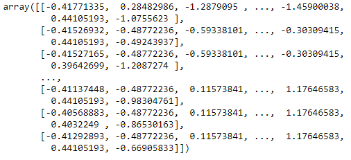
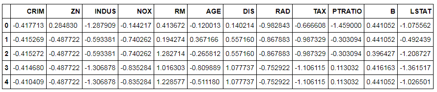
We convert the above output, which is in array format, into a DataFrame.

Scaled_BosData = pd.DataFrame(BosData_scaled,columns=BosData_Scaled.columns)
Scaled_BosData.head()

Show full table ▾

In this step, we concatenate the scaled variables with the leftover categorical variable.

BosData_chas = BosData[['CHAS']]
BosData_Final = pd.concat([BosData_chas,Scaled_BosData],axis=1)

Splitting Dataset into Train and Test

Here we split the dataset into Train and Test. Note that these datasets will be used again when we deal with KNN.

X1_train,X1_test,Y1_train,Y1_test=train_test_split(BosData_Final,BosData['ln_Price'],test_size=0.3,random_state=123)

Lasso

Initialize and Fit Model: We build a Lasso Regression model, which uses an l1 penalty, and fit it on the Train dataset.

Lasso = linear_model.Lasso(alpha=0.01)
Lasso.fit(X1_train,Y1_train)

Prediction and Calculate Accuracy: In this step, we predict the dependent variable on the Test dataset and calculate its R².

pred1 = Lasso.predict(X1_test)
metrics.r2_score(Y1_test,pred1)

The accuracy of this model comes out to be 67%.

Ridge

Building and Fitting Model: We build the Ridge Regression model and fit it on the Train dataset.

Ridge = linear_model.Ridge()
Ridge.fit(X1_train,Y1_train)

Find Coefficients: We can use the Ridge.coef_ command to see the coefficients derived from this Ridge Regression model.

Ridge.coef_

Prediction: We predict the dependent variable on the Test dataset.

ridge_test_pred = pd.DataFrame({'actual':Y1_test,'predicted':Ridge.predict(X1_test)})

Calculate Accuracy: We now calculate the accuracy, to compare results with the simple Linear and Lasso Regression models.

score_Ridge = metrics.r2_score(ridge_test_pred['actual'],ridge_test_pred['predicted'])
score_Ridge

The accuracy provided by Ridge is 71%, which is more than that of Lasso.

Elastic Net

For Regression, we use the ElasticNet model, whereas for Classification we use the Stochastic Gradient Descent Classifier.

Import Library: Here we import linear_model from scikit-learn to create an Elastic Net Regression model.

from sklearn import linear_model

Initialize Model: In this step we use linear_model.ElasticNet and initialize the model, setting the alpha value at 0.01.

EN = linear_model.ElasticNet(alpha=0.01)

Fit Model: We now fit the model on the Train dataset.

EN.fit(X1_train,Y1_train)

Prediction: We predict the dependent variable on the Test dataset.

pred_EN = EN.predict(X1_test)

Calculate Accuracy: We now calculate the accuracy of the Elastic Net Regression model.

metrics.r2_score(Y1_test,pred_EN)

This model provides us with 69% accuracy.

Tuning of Parameters

We will now tune the parameters for Regularized Regression using Grid Search and Random Search. As discussed above, these methods will run the model with various parameters and provide us with the best parameter values. Here we look for the best value of alpha, and upon finding it we fit the model on the Train dataset, predict the values on the Test dataset, and calculate the accuracy score using the metrics package. For Elastic Net, we additionally tune a parameter called l1_ratio, the ElasticNet mixing parameter, whose value is taken between 0 and 1.

Grid Search - Ridge

Import GridSearchCV Library: We import GridSearchCV from sklearn.model_selection, which we will use to tune hyperparameters.

from sklearn.model_selection import GridSearchCV

Defining Parameters: Parameters have to be defined first before they can be used in Grid Search. The range of parameters is defined differently in Grid Search and Random Search - Grid Search requires discrete values, whereas Random Search uses a range of values for parameters.

params_Ridge = {'alpha': np.array([1,0.1,0.01,0.001,0.0001,0])}

Building and Fitting Model: We now build the Regularized Linear Regression model using Grid Search and fit it on the Train dataset.

Ridge_GS = GridSearchCV(Ridge, param_grid=params_Ridge)
Ridge_GS.fit(X1_train,Y1_train)

Best Parameters: The best_params_ command can be used to find the best parameters.

Ridge_GS.best_params_

The best value of alpha is considered to be 1.

Prediction: We predict the house prices on the Test dataset.

pred_Ridge_GS = Ridge_GS.predict(X1_test)

Calculate Accuracy: We now compute the accuracy of this model.

metrics.r2_score(Y1_test,pred_Ridge_GS)

The accuracy comes out to be 71%.

Note - here we have used Ridge Regression. You can perform the same steps mentioned above for hyperparameter tuning of a Lasso Regression model.

Grid Search - Elastic Net

Defining Parameters: For the Elastic Net Regression model, we will tune two parameters: alpha and l1_ratio.

params_EN = {'alpha' :np.array([1,0.1,0.01,0.001,0.0001,0]),
         'l1_ratio' :np.array([0.1,0.01,0.001,0.0001,1])}

Building and Fitting Model: We now build the model using Grid Search and fit it on the Train dataset.

EN_GS = GridSearchCV(linear_model.ElasticNet(), param_grid=params_EN)
EN_GS.fit(X1_train,Y1_train)

Best Parameters: The best_params_ command can be used to find the best parameters.

EN_GS.best_params_

Prediction: We now predict using this model on the Test dataset.

pred_EN_GS = EN_GS.predict(X1_test)

Calculate Accuracy: We compute the accuracy of this Elastic Net Regression model.

metrics.r2_score(Y1_test,pred_EN_GS)

The accuracy comes out to be 71%.

Random Search - Ridge

Import RandomizedSearchCV Library: We import RandomizedSearchCV from sklearn.model_selection, which will allow us to tune hyperparameters.

from sklearn.model_selection import RandomizedSearchCV

Declaring Parameters: As the values of alpha can be in decimals, we use a uniform distribution to define the range of the parameter alpha, importing uniform from scipy.stats. For integers we can use sp_randint, which takes random integer values in a range. Here we import uniform from scipy.stats and declare a list of plausible parameters.

from scipy.stats import uniform
params_Ridge_RS = {'alpha': uniform(0.0001,1)}

Building Model: We build the model and search for the best parameters. Here we run 100 iterations to come up with the best value of the parameter.

Ridge_RS = RandomizedSearchCV(Ridge, param_distributions=params_Ridge_RS,n_iter=100)

Fitting Model: We now fit the model on the Train dataset.

Ridge_RS.fit(X1_train,Y1_train)

Best Parameters: The best_params_ command can be used to find the best parameters.

Ridge_RS.best_params_

The best value of alpha is considered to be 0.9937662069031356.

Predict and Check Accuracy: The above model is used to predict the values of the dependent variable on the Test dataset, and the accuracy is also calculated.

pred_Ridge_RS = Ridge_RS.predict(X1_test)
metrics.r2_score(Y1_test,pred_Ridge_RS)

The accuracy comes out to be 71%, the same as when we used alpha=1, which was provided by Grid Search.

Note - here we had used Ridge Regression. You can perform the same steps mentioned above for hyperparameter tuning of a Lasso Regression model.

Random Search - Elastic Net

Defining Parameters: We provide a distribution of values for the two hyperparameters.

params_EN_RS = {'alpha': uniform(0.0001,1),
               'l1_ratio':uniform(0.0001,1) }

Building and Fitting Model: We now build a model using RandomizedSearchCV and fit it on the Train dataset.

EN_RS = RandomizedSearchCV(linear_model.ElasticNet(), param_distributions=params_EN_RS,n_iter=100)
EN_RS.fit(X1_train,Y1_train)

Best Parameters: We use the best_params_ command and check for the best parameters obtained from RandomizedSearchCV.

EN_RS.best_params_

Predict and Check Accuracy: The above model is used to predict the values of the dependent variable on the Test dataset. In this step, we also check the accuracy obtained by the model.

pred_EN_RS = EN_RS.predict(X1_test)
metrics.r2_score(Y1_test,pred_EN_RS)

We get 70% accuracy from the above model.

Decision Tree Regressor

Decision Trees allow us to come up with flowcharts structured as trees, which allow us to predict the value of the dependent variable. Their inner workings have been explained in Decision Trees under the Theory Section.

This algorithm does not require scaled data, so we use the same Train and Test dataset components as used in the Linear Regression model: X_train, Y_train, X_test and Y_test.

Importing Libraries

We import DecisionTreeRegressor from sklearn.tree, which allows us to create a Decision Tree Regression model.

from sklearn.tree import DecisionTreeRegressor

Initializing and Fitting Decision Tree Model

Here we initialize the Decision Tree model. We are using no hyperparameters and simply use DecisionTreeRegressor() to initialize, and then fit this model on the Train dataset.

DTR = DecisionTreeRegressor()
DTR.fit(X_train,Y_train)

Prediction and Calculating Accuracy

The Decision Tree model is used to predict the Y variable on the Test dataset. We also check the accuracy of this model on the Test dataset.

Pred_DTR = DTR.predict(X_test)
metrics.r2_score(Y_test,Pred_DTR)

The accuracy of this Decision Tree model comes out to be 66%.

Tree Visualization

We can visualize the above-created Decision Tree. This helps in further understanding how the decision tree algorithm is working.

Install and Import graphviz: We have to install graphviz in Python by typing pip install graphviz in the command window. Once done, we can import the graphviz library in Python.

import graphviz

Creating Decision Tree Visualization: We now import tree from scikit-learn and then use graphviz to create the Decision Tree flowchart.

dot_data = tree.export_graphviz(DTR, out_file=None)
graph = graphviz.Source(dot_data)
graph.render("train_set1")

Decision Tree with Labels: The above command produces a decision tree flowchart without variable names, so we use the following code to produce the decision tree flowchart with variable names.

dot_data = tree.export_graphviz(DTR, out_file=None, max_depth=3,
                               feature_names=X.columns,
                         filled=True, rounded=True,
                         special_characters=True)
graph2 = graphviz.Source(dot_data)
graph2.render('train_setlinear')

Opening Saved Image: We import os and use the os.startfile command to open the PDF file of the tree chart.

import os
os.startfile('train_setlinear')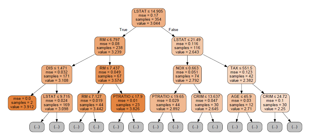

Tuning Hyperparameters

To show an example of how hyperparameters can be tuned, we take the following four parameters: max_features, the number of features to be considered when looking for the best split; the minimum sample split; the minimum sample leaf; and max_depth, the maximum depth of the tree. All such hyperparameters have been explained in the Theory Section. You may select other parameters if you want more control over the process and desire more accuracy.

Grid Search

Defining Parameters: Here we define the plausible values for our four parameters.

params = {'max_features': ['auto', 'sqrt', 'log2'],
          'min_samples_split': [2,3,4,5,6,7,8,9,10,11,12,13,14,15],
          'min_samples_leaf':[1,2,3,4,5,6,7,8,9,10,11],
         'max_depth':[2,3,4,5,6,7,8]}

Initializing Decision Tree: We now initialize the Decision Tree Regression model.

DTR = DecisionTreeRegressor()

Building and Fitting Model: We now build a model using GridSearchCV and fit it on the Train dataset.

DTR_GS = GridSearchCV(DTR, param_grid=params)
DTR_GS.fit(X_train,Y_train)

Best Parameters: The best_params_ command can be used to find the best parameters.

DTR_GS.best_params_

Predict and Check Accuracy: The above model, with the values of hyperparameters found above, is used to predict the values of the dependent variable on the Test dataset, and the accuracy is also calculated.

pred_DTR_GS = DTR_GS.predict(X_test)
metrics.r2_score(Y_test,pred_DTR_GS)

The accuracy comes out to be 68%.

Random Search

Defining Parameters: As mentioned earlier, for parameters that are integers we use sp_randint, which we import from scipy.stats.

from scipy.stats import randint as sp_randint

param_grid2 = {'max_features': ['auto', 'sqrt', 'log2'],
          'min_samples_split': sp_randint(2,15),
          'min_samples_leaf': sp_randint(1,11),
          'max_depth':sp_randint(2,8)}

Building and Fitting Model: We now build a model using RandomizedSearchCV and fit it on the Train dataset.

DTR_RS = RandomizedSearchCV(DTR, param_distributions=param_grid2,n_iter=100)
DTR_RS.fit(X_train,Y_train)

Best Parameters: We use the best_params_ command and check for the best parameters obtained from RandomizedSearchCV.

DTR_RS.best_params_

Predict and Check Accuracy: The above model with the best parameters is used to predict the values of the dependent variable on the Test dataset, and the accuracy is also calculated.

pred_DTR_RS = DTR_RS.predict(X_test)
metrics.r2_score(Y_test,pred_DTR_RS)

The accuracy comes out to be 68%.

K Nearest Neighbour

KNN is a distance-based algorithm which predicts a value based on the number of class observations found in its neighbourhood. For a detailed understanding of KNN, refer to K Nearest Neighbour under the Theory Section.

Importing KNeighborsRegressor Package

To run KNN in Python, we require KNeighborsRegressor, which we import from sklearn.neighbors.

from sklearn.neighbors import KNeighborsRegressor

Initializing and Fitting KNN Model

In this step, we first initialize the KNN model and then fit it on the Train dataset. Note that this is the Train dataset we used earlier for Regularized Regression - as discussed above, KNN requires standardized data, since it uses distance as a parameter for its functioning. We therefore use a dataset with all numerical observations scaled, except the target variable, using the same datasets as used for Regularized Regression to predict the value of Price on the Test dataset.

knnr = KNeighborsRegressor()
knnr.fit(X1_train,Y1_train)

Predict and Check Accuracy

The above model is used to predict the values of the dependent variable on the Test dataset, and the accuracy is calculated.

pred_knnr = knnr.predict(X1_test)
metrics.r2_score(Y1_test,pred_knnr)

The accuracy comes out to be 76%.

Tuning Hyperparameters

In this blog post, we will tune four hyperparameters for KNN: n_neighbors, where we declare the different numbers of neighbours that can be considered; algorithm, where we can use methods such as K-D trees, which help speed up the testing phase; leaf_size, which helps the algorithm decide when to switch from the usual brute force method to tree-based methods such as K-D trees; and weights, where alternatives to majority voting can be provided. (All such hyperparameters have been explained in the theoretical explanation of KNN, so one can refer to it for more information. There are also a number of other hyperparameters to choose from, which you may select if you want more control over the process and desire more accuracy.)

Grid Search

Defining Parameters: We define the values for our four parameters.

params_knn = {'n_neighbors':[5,6,7,8,9,10],
          'leaf_size':[1,2,3,5],
          'weights':['uniform', 'distance'],
          'algorithm':['auto', 'ball_tree','kd_tree','brute']}

Building and Fitting Model: We now build a KNN model using GridSearchCV and fit it on the Train dataset.

model_knn1 = GridSearchCV(knnr, param_grid=params_knn)
model_knn1.fit(X1_train,Y1_train)

Best Parameters: We use best_params_ to check for the best parameters.

model_knn1.best_params_

Predict and Check Accuracy: The above model, with the above-mentioned values of hyperparameters, is used to predict the values of the dependent variable on the Test dataset, and the accuracy is also calculated.

pred_knnr_GS = model_knn1.predict(X1_test)
metrics.r2_score(Y1_test,pred_knnr_GS)

The accuracy obtained from this model is 78%.

Random Search

Defining Parameters: We define a range of values for our four parameters.

params_knn_rs = {'n_neighbors':sp_randint(5,10),
          'leaf_size':sp_randint(1,5),
          'weights':['uniform', 'distance'],
          'algorithm':['auto', 'ball_tree','kd_tree','brute']}

Building and Fitting Model: We now build a KNN model using RandomizedSearchCV and fit it on the Train dataset.

KNN_RS1 = RandomizedSearchCV(knnr, param_distributions=params_knn_rs,n_iter=100)
KNN_RS1.fit(X1_train,Y1_train)

Best Parameters: We now check for the best parameters obtained using Random Search.

KNN_RS1.best_params_

Predict and Check Accuracy: We use the above model and the best combination of hyperparameters to predict the values of the dependent variable on the Test dataset, and the accuracy is also calculated.

pred_knn_RS = KNN_RS1.predict(X1_test)
metrics.r2_score(Y1_test,pred_knn_RS)

The accuracy comes out to be 78%.

Ensemble Models

In the Theory Section, under Ensemble Methods, various kinds of ensemble techniques have been explored. Here we will explore all those ensemble techniques using Python.

Bagging Regressor

Bagging Regressor is an ensemble estimator which fits a base estimator on each random subset of the Train dataset, and then aggregates their individual predictions to form a final prediction using a voting or averaging method. Here the base estimator is Decision Trees.

Importing BaggingRegressor Library

To create a Bagging Regressor model in Python, we import BaggingRegressor from sklearn.ensemble.

from sklearn.ensemble import BaggingRegressor

Initializing and Fitting Model

We initialize the Bagging model and fit it on the Train dataset.

baggingR = BaggingRegressor()
baggingR.fit(X_train,Y_train)

Note that if base_estimator is None, the base estimator is a Decision Tree. bootstrap tells the model whether to draw samples with replacement; bootstrap_features is for whether features are drawn with replacement.

Predict and Check Accuracy

The above model is used to predict the values of the dependent variable on the Test dataset and check its accuracy.

bag_test_pred = baggingR.predict(X_test)
metrics.r2_score(Y_test,bag_test_pred)

The accuracy obtained from this Bagging Regression model is 82%.

Tuning Hyperparameters

Here we tune five parameters: n_estimators, max_features, max_samples, bootstrap and bootstrap_features.

Grid Search

Defining Parameters: Here we define our five parameters.

params_bag_GS = {"n_estimators": [50,100,200],
               "max_features":[1,2,4,6,8],
               "max_samples": [0.5,0.1],
             "bootstrap": [True, False],
          "bootstrap_features": [True, False]}

Initializing, Building and Fitting Model: In this step, we initialize and build the Bagging Regression model using GridSearchCV and fit it on the Train dataset.

Bag_model_GS = GridSearchCV(baggingR, param_grid=params_bag_GS)
Bag_model_GS.fit(X_train,Y_train)

Best Parameters: We now check the best combination of parameters.

Bag_model_GS.best_params_

Predict and Check Accuracy: We use this model to predict the dependent variable on the Test dataset and check its accuracy.

pred_bag_GS = Bag_model_GS.predict(X_test)
metrics.r2_score(Y_test,pred_bag_GS)

The accuracy comes out to be 82%.

Random Search

Defining Parameters: We provide a distribution of values for the five hyperparameters.

params_bagR_RS = {"n_estimators": sp_randint(50,200),
              "max_features":sp_randint(1,8),
              "max_samples": uniform(0.5,0.1),
            "bootstrap": [True, False],
         "bootstrap_features": [True, False]}

Building and Fitting Model: We now build a model using RandomizedSearchCV and fit it on the Train dataset.

BagR_RS = RandomizedSearchCV(baggingR, param_distributions=params_bagR_RS,n_iter=120)
BagR_RS.fit(X_train,Y_train)

Best Parameters: We use the best_params_ command and check for the best parameters obtained from RandomizedSearchCV.

BagR_RS.best_params_

Predict and Check Accuracy: The above model is used to predict the values of the dependent variable on the Test dataset. In this step we also check the accuracy obtained by the model.

pred_bagR_RS = BagR_RS.predict(X_test)
metrics.r2_score(Y_test,pred_bagR_RS)

The accuracy comes out to be 83%.

Random Forest Regressor

Random Forest Regressor is a variant of Bagging Regressor, and more about it can be found in the blog Bagging available in the Theory Section.

Importing RandomForestRegressor Library

We have to import RandomForestRegressor from sklearn.ensemble to run a Random Forest Regression model.

from sklearn.ensemble import RandomForestRegressor

Initializing and Fitting Model

We initialize the Random Forest model and then fit it on the Train dataset.

rfr = RandomForestRegressor()
rfr.fit(X_train,Y_train)

Predict and Check Accuracy

The above model is used to predict the values of the dependent variable on the Test dataset. We also check the model's performance.

rfr_test_pred = rfr.predict(X_test)
metrics.r2_score(Y_test, rfr_test_pred)

The accuracy obtained from this Random Forest Regression model is 79%.

Tuning Hyperparameters

Here we tune four parameters: max_depth, max_features, min_samples_split and min_samples_leaf.

Grid Search

Defining Parameters: First, we define our four parameters.

params_RF = {"max_depth": [3,5,6,7,8,9],
              "max_features":['auto', 'sqrt', 'log2'],
              "min_samples_split": [2, 3,5,7],
              "min_samples_leaf": [1, 3,5,6]}

Initializing, Building and Fitting Model: In this step, we initialize and build the Random Forest Regression model using GridSearchCV and fit it on the Train dataset.

model_RF_GS = GridSearchCV(rfr, param_grid=params_RF)
model_RF_GS.fit(X_train,Y_train)

Best Parameters: We now check for the best combination of parameters.

model_RF_GS.best_params_

Predict and Check Accuracy: We use this model to predict the dependent variable on the Test dataset and check its accuracy.

pred_RF_GS = model_RF_GS.predict(X_test)
metrics.r2_score(Y_test,pred_RF_GS)

The accuracy comes out to be 79%.

Random Search

Defining Parameters: We provide a distribution of values for the four hyperparameters.

params_RF_RS = {"max_depth": sp_randint(3,9),
              "max_features":['auto', 'sqrt', 'log2'],
              "min_samples_split":sp_randint(2,7),
              "min_samples_leaf": sp_randint(1,6)}

Building and Fitting Model: We now build a model using RandomizedSearchCV and fit it on the Train dataset.

rfr_RS = RandomizedSearchCV(rfr, param_distributions=params_RF_RS,n_iter=100)
rfr_RS.fit(X_train,Y_train)

Best Parameters: We use the best_params_ command and check for the best parameters obtained from RandomizedSearchCV.

rfr_RS.best_params_

Predict and Check Accuracy: The above model is used to predict the values of the dependent variable on the Test dataset. In this step, we also check the accuracy obtained by the model.

pred_RF_RS = rfr_RS.predict(X_test)
metrics.r2_score(Y_test,pred_RF_RS)

The accuracy comes out to be 80%.

AdaBoost Regressor

The AdaBoost Regressor builds a regressor (decision tree), and if a training data point is mispredicted, the weight of that training data point is increased, i.e. it is boosted. Here again, Decision Tree Regressor is used as the base estimator.

Importing AdaBoostRegressor Package

We require AdaBoostRegressor, which we import from sklearn.ensemble, to create an AdaBoost Regression model.

from sklearn.ensemble import AdaBoostRegressor

Initializing and Fitting AdaBoost Model

In this step, we first initialize the AdaBoost model, and then fit this model on the Train dataset.

AdaBoost = AdaBoostRegressor()
AdaBoost.fit(X_train,Y_train)

Predict and Check Accuracy

The above model is used to predict the values of the dependent variable on the Test dataset, and the accuracy is calculated.

AdaBoost_test_pred = AdaBoost.predict(X_test)
metrics.r2_score(Y_test,AdaBoost_test_pred)

The accuracy comes out to be 78%.

Tuning Hyperparameters

In this blog post, we will tune the number of estimators and the learning rate.

Grid Search

Defining Parameters: We first define the values for our parameters.

params_AdbR_GS = {'learning_rate':[0.05,0.1,0.2,0.6,0.8,1],
        'n_estimators': [50,60,100],
                 'loss' : ['linear', 'square', 'exponential']}

Building and Fitting Model: We now build an AdaBoost model using GridSearchCV and fit it on the Train dataset.

model_AdaR_GS = GridSearchCV(AdaBoostRegressor(), param_grid=params_AdbR_GS)
model_AdaR_GS.fit(X_train,Y_train)

Best Parameters: We use the best_params_ function to check for the best parameters.

model_AdaR_GS.best_params_

Predict and Check Accuracy: The above model, with the above-mentioned values of hyperparameters, is used to predict the values of the dependent variable on the Test dataset, and the accuracy is also calculated.

pred_AdaR_GS = model_AdaR_GS.predict(X_test)
metrics.r2_score(Y_test,pred_AdaR_GS)

The accuracy obtained from this model is 78%.

Random Search

Defining Parameters: We define a range of values for our two parameters.

params_AdbR_RS = {'learning_rate':uniform(0.05,1),
        'n_estimators': sp_randint(50,100),
                'loss' : ['linear', 'square', 'exponential']}

Building and Fitting Model: We now build an AdaBoost model using RandomizedSearchCV and fit it on the Train dataset.

AdaR_RS = RandomizedSearchCV(AdaBoostRegressor(), param_distributions=params_AdbR_RS,n_iter=100)
AdaR_RS.fit(X_train,Y_train)

Best Parameters: We now check for the best parameters obtained using Random Search.

AdaR_RS.best_params_

Predict and Check Accuracy: We use the above model and the best combination of hyperparameters to predict the values of the dependent variable on the Test dataset, and the accuracy is also calculated.

pred_AdaR_RS = AdaR_RS.predict(X_test)
metrics.r2_score(Y_test,pred_AdaR_RS)

The accuracy comes out to be 78%.

Gradient Boosting Regressor

Gradient Boosting Regressor is another type of Boosting Model. Refer to the blog Boosting under Ensemble Methods in the Theory Section to know more about it.

Importing GradientBoostingRegressor Library

To create a Gradient Boost Regression model in Python, we require importing GradientBoostingRegressor from sklearn.ensemble.

from sklearn.ensemble import GradientBoostingRegressor

Initializing and Fitting Model

We initialize the model and fit it on the Train dataset.

GBR = GradientBoostingRegressor()
GBR.fit(X_train,Y_train)

Predict and Check Accuracy

The above model is used to predict the values of the dependent variable on the Test dataset and check its accuracy.

GBR_test_pred = GBR.predict(X_test)
metrics.r2_score(Y_test, GBR_test_pred)

The accuracy obtained from this Gradient Boosting Regression model is 84%.

Tuning Hyperparameters

Here we tune six parameters: max_depth, max_features, min_samples_split, min_samples_leaf, learning_rate and n_estimators.

Grid Search

Defining Parameters: Here we define our six parameters.

params_GBR_GS = {"max_depth": [3,5,6,7],
              "max_features":['auto', 'sqrt', 'log2'],
              "min_samples_split": [2, 3, 10],
              "min_samples_leaf": [1, 3, 10],
            'learning_rate':[0.05,0.1,0.2],
            'n_estimators': [10,30,50,70]}

Initializing, Building and Fitting Model: In this step, we initialize and build the Gradient Boosting Regression model using GridSearchCV and fit it on the Train dataset.

model_GradR2_GS = GridSearchCV(GradientBoostingRegressor(), param_grid=params_GBR_GS)
model_GradR2_GS.fit(X_train,Y_train)

Best Parameters: We now check the best combination of parameters.

model_GradR2_GS.best_params_

Predict and Check Accuracy: We use this model to predict the dependent variable on the Test dataset and check its accuracy.

pred_GradR_GS = model_GradR2_GS.predict(X_test)
metrics.r2_score(Y_test,pred_GradR_GS)

The accuracy comes out to be 86%.

Random Search

Defining Parameters: We provide a distribution of values for the six hyperparameters.

params_GBR_RS = {"max_depth":sp_randint(3,7),
              "max_features":['auto', 'sqrt', 'log2'],
              "min_samples_split": sp_randint(2,10),
              "min_samples_leaf": sp_randint(1,10),
                'learning_rate':uniform(0.05,0.2),
                'n_estimators':sp_randint(10,70)}

Building and Fitting Model: We now build a model using RandomizedSearchCV and fit it on the Train dataset.

GradR_RS = RandomizedSearchCV(GradientBoostingRegressor(), param_distributions=params_GBR_RS,n_iter=100)
GradR_RS.fit(X_train,Y_train)

Best Parameters: We use the best_params_ command and check for the best parameters obtained from RandomizedSearchCV.

GradR_RS.best_params_

Predict and Check Accuracy: The above model is used to predict the values of the dependent variable on the Test dataset. In this step we also check for the accuracy obtained by the model.

pred_GradR_RS = GradR_RS.predict(X_test)
metrics.r2_score(Y_test,pred_GradR_RS)

The accuracy comes out to be 85%.

XGBoost Regressor

XGBoost stands for Extreme Gradient Boost, which is an advanced version of Gradient Boost.

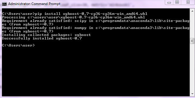
Installing and Importing Library

We first download the file xgboost-0.7-cp36-cp36m-win_amd64.whl from https://www.lfd.uci.edu/~gohlke/pythonlibs/#xgboost and install the file using the command prompt, as shown below.

We now import XGBRegressor from xgboost to run an Extreme Gradient Boosting model.

from xgboost import XGBRegressor

Initializing and Fitting Model

We initialize the model and fit it on the Train dataset.

xgbr = XGBRegressor()
xgbr.fit(X_train,Y_train)

Prediction and Accuracy

The above model is used to predict the values of the dependent variable on the Test dataset. We also check the model's performance.

pred_xgbr = xgbr.predict(X_test)
metrics.r2_score(Y_test,pred_xgbr)

The accuracy obtained from this XGBoost Regression model is 85%.

Tuning Hyperparameters

Here we tune four parameters: max_depth, min_child_weight, learning_rate and n_estimators.

Grid Search

Defining Parameters: First, we define our four parameters.

params_xgbR_GS = {"max_depth": [3,4,5,6,7,8],
              "min_child_weight" : [4,5,6,7,8],
            'learning_rate':[0.05,0.1,0.2,0.25,0.8,1],
            'n_estimators': [10,30,50,70,80,100]}

Initializing, Building and Fitting Model: In this step, we initialize and build the Extreme Gradient Regression model using GridSearchCV and fit it on the Train dataset. We also import warnings and run filterwarnings so that any unnecessary warning can be ignored.

import warnings
warnings.filterwarnings("ignore")

model_xgbR_GS = GridSearchCV(XGBRegressor(), param_grid=params_xgbR_GS)
model_xgbR_GS.fit(X_train,Y_train)

Best Parameters: We now check for the best combination of parameters.

model_xgbR_GS.best_params_

Predict and Check Accuracy: We use this model to predict the dependent variable on the Test dataset and check its accuracy.

pred_xgbR_GS = model_xgbR_GS.predict(X_test)
metrics.r2_score(Y_test,pred_xgbR_GS)

The accuracy comes out to be 84%.

Random Search

Defining Parameters: We provide a distribution of values for the four hyperparameters.

params_xgbR_RS = {"max_depth":sp_randint(3,8),
              "min_child_weight" : sp_randint(4,8),
            'learning_rate':uniform(0.05,1),
            'n_estimators':sp_randint(10,100)}

Building and Fitting Model: We now build a model using RandomizedSearchCV and fit it on the Train dataset.

XGB_RS = RandomizedSearchCV(XGBRegressor(), param_distributions=params_xgbR_RS,n_iter=150)
XGB_RS.fit(X_train,Y_train)

Best Parameters: We use the best_params_ command and check for the best parameters obtained from RandomizedSearchCV.

XGB_RS.best_params_

Predict and Check Accuracy: The above model is used to predict the values of the dependent variable on the Test dataset. In this step, we also check for the accuracy obtained by the model.

pred_xgb_RS = XGB_RS.predict(X_test)
metrics.r2_score(Y_test,pred_xgb_RS)

We get 85% accuracy from this model.

Stacking Regressor

Stacking is a method where we use multiple learning algorithms and get a result by combining the results of all these separate algorithms. In this blog, we will perform a Level-One stacking. To know more about it, refer to the blog Stacking under the Theory Section.

Importing Library

We import StackingRegressor, which will allow us to create a stacked regression model.

from mlxtend.regressor import StackingRegressor

Initiating Individual Models

We now initiate all the models that we require in the Level-0 and in the meta-layer of the stacked model.

mod1 = KNeighborsRegressor()
mod2 = RandomForestRegressor()
mod3 = Ridge()
lr = LinearRegression()

Initiating the Stacked Model

We finally initiate the stacked model, having KNN, Random Forest, Ridge Regression and Linear Regression in the level-0, and the Linear Regressor in the meta-layer.

sr = StackingRegressor(regressors=[mod1, mod2,mod3 ,lr],
                          meta_regressor=lr)

Fitting Model

We fit the stacked regression model on the Train dataset.

sr.fit(X_train,Y_train)

Predicting and Checking Accuracy

We now predict the dependent variable on the Test dataset and, on the basis of these predictions, check the accuracy of this stacked model.

sr_pred = sr.predict(X_test)
metrics.r2_score(Y_test,sr_pred)

We get a 79% accuracy from this model.

In this blog, we explored the various regression algorithms covered in the Theory Section of Modeling. All such algorithms have been put to use using R in the blog Regression Problems in R.