// application · python

Feature Engineering in Python

Various concepts of Feature Engineering have been explored in the Theory section. In this blog, we will discuss how to apply those concepts to datasets using Python. The following topics will be covered in this blog:

• Feature Transformation
• Feature Scaling
• Feature Construction
• Feature Reduction

Feature Transformation

Import Dataset: To explore Feature Transformation, we will use the CarData dataset and look at the variable 'Sales_in_thousands'.

CarData = pd.read_excel("C:/Users/user/Desktop/Data Sets/Car_Data1.xls")

Checking Skewness: We first check the skewness of the variable 'Sales_in_thousands'.

CarData['Sales_in_thousands'].skew()

We plot a histogram to see the distribution of the variable visually.

CarData['Sales_in_thousands'].hist()

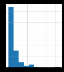
We can see that the variable is highly positively skewed. We will now apply various transformations to normalize this variable.

Log Transformation

We apply a Log Transformation to the variable and check the skewness again.

log_transform = np.log(CarData['Sales_in_thousands'])
log_transform.skew()

log_transform.hist()

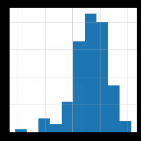
We see that the Log Transformation has overcorrected the skewness, and the variable is now negatively skewed.

Square-Root Transformation

We apply a Square-Root Transformation to the variable and check the skewness again.

sqrt_transform = np.sqrt(CarData['Sales_in_thousands'])
sqrt_transform.skew()

sqrt_transform.hist(color="orange")

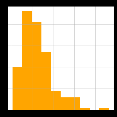
The skewness has reduced compared to the original variable, however, the variable is still positively skewed.

Cube-Root Transformation

We apply a Cube-Root Transformation to the variable and check the skewness again.

cbrt_transform = np.cbrt(CarData['Sales_in_thousands'])
cbrt_transform.skew()

cbrt_transform.hist(color="green")

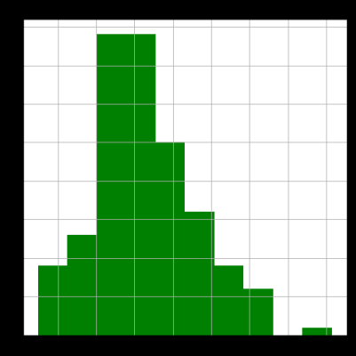
Out of the three transformations explored above, the Cube-Root Transformation gives us the value of skewness closest to zero, and therefore is the most suitable transformation for this variable among the three.

Feature Scaling

Import Dataset: To explore Feature Scaling, we use a dataset having the Income and Age of 10 people.

IncAgeData = pd.read_excel("C:/Users/user/Desktop/Data Sets/IncAgeData.xls")
IncAgeData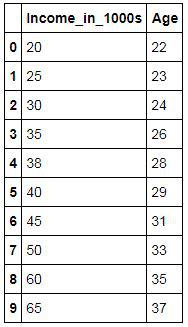

Min-Max Scaler

We use the MinMaxScaler from sklearn to scale the dataset between 0 and 1.

from sklearn.preprocessing import MinMaxScaler
scaler = MinMaxScaler()
scaled = scaler.fit_transform(IncAgeData)
scaled

We see that the Min-Max Scaler has scaled the dataset such that the minimum value of each variable becomes 0 and the maximum value becomes 1, with all other values scaled proportionately in between.

Z-Score (Standardization)

We use sklearn.preprocessing to standardize the variable 'Income_in_1000s' by calculating its Z-Score.

We first calculate the mean of the variable.

IncAgeData['Income_in_1000s'].mean()

We then calculate the sample standard deviation of the variable.

IncAgeData['Income_in_1000s'].std()

We use the scale function from sklearn to calculate the Z-Score directly.

from sklearn.preprocessing import scale
z_score = scale(IncAgeData['Income_in_1000s'])
z_score

We can also convert this output into a Series for ease of viewing.

z_score = pd.Series(z_score)
z_score

Feature Construction

Binning

Import Dataset: To explore Binning, we use the Height dataset having the height of 20 people.

HeightData = pd.read_excel('C:/Users/user/Desktop/Data Sets/Height_Data1.xls')
HeightData

Show full table ▾

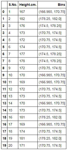
Automatic Binning

We use the cut function from pandas to automatically create 4 equal-width bins for the variable 'Height.cm.'.

HeightData['Bins'] = pd.cut(HeightData['Height.cm.'],4)
HeightData

Show full table ▾

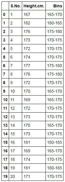
Manual Binning

Import Dataset: We use the same Height dataset to perform manual binning, this time specifying our own bin edges.

HeightData2 = pd.read_excel('C:/Users/user/Desktop/Data Sets/Height_Data1.xls')
HeightData2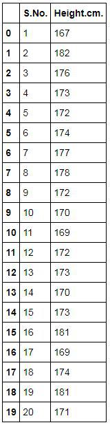

Show full table ▾

We specify our own bin edges and labels and apply them using the cut function.

bins = [165,170,175,180,185]
labels = ['165-170','170-175','175-180','180-185']
HeightData2['Bins'] = pd.cut(HeightData2['Height.cm.'],bins=bins,labels=labels)
HeightData2

Show full table ▾

Encoding

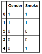
Import Dataset: We use a small dataset having a categorical variable 'a' (Gender) and a numeric variable 'b'.

Encode1 = pd.DataFrame({'a':['M','F','F','M','M','F','M','F','M','F'],'b':[22,23,24,26,28,30,27,32,35,37]})
Encode1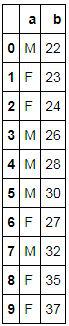

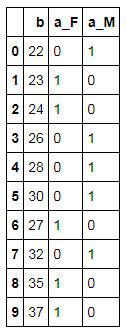
Get Dummies

We use the get_dummies function from pandas to one-hot encode the categorical variable 'a'.

Encode2 = pd.get_dummies(Encode1,columns=['a'])
Encode2

Import Dataset: We now use a larger dataset, having information on the Gender and Smoking status of 19 people, to further explore encoding.

SmokingData2 = pd.read_excel("C:/Users/user/Desktop/Data Sets/SmokingData2.xls")
SmokingData2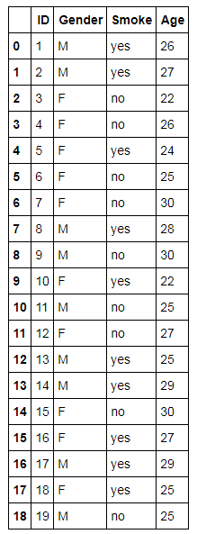

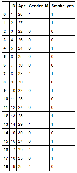
Show full table ▾

Get Dummies with drop_first: We use drop_first=True to avoid the dummy variable trap by dropping the first category of each encoded variable.

SmokingData3 = pd.get_dummies(SmokingData2,columns=['Gender','Smoke'],drop_first=True)
SmokingData3

Show full table ▾

One-Hot Encoding using sklearn

We now perform One-Hot Encoding using the OneHotEncoder and LabelEncoder classes from sklearn.preprocessing.

from sklearn.preprocessing import LabelEncoder, OneHotEncoder
label_encoder = LabelEncoder()

We first label-encode the variable 'Gender' into integers.

integer_encoded = label_encoder.fit_transform(SmokingData2['Gender'])
integer_encoded

We then use OneHotEncoder to convert these integer labels into a one-hot encoded array.

onehot_encoder = OneHotEncoder(sparse_output=False)
integer_encoded = integer_encoded.reshape(len(integer_encoded), 1)
onehot_encoded = onehot_encoder.fit_transform(integer_encoded)
onehot_encoded

One-Hot Encoding on Dataset

We now perform One-Hot Encoding on the dataset that we used above during the application of the get_dummies function.

Separate Categorical Variables and perform Labeling: We first separate the categorical variables from the dataset and then label them.

SData3 = SmokingData2[['Gender','Smoke']]
int_lab = SData3.apply(label_encoder.fit_transform)
int_lab.head()

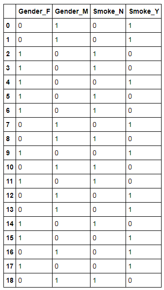
Perform One-Hot Encoding on Dataset: We now perform One-Hot Encoding on these categorical labelled variables.

Onhotencode = OneHotEncoder(sparse_output=False,dtype=int)
one_hot_encode_output = Onhotencode.fit_transform(int_lab)
one_hot_encode_output

Transforming the output into Dataframe: For our convenience and ease, we transform the above output into a Dataframe.

one_hot_encode_output1 = pd.DataFrame(one_hot_encode_output,columns=['Gender_F','Gender_M','Smoke_N','Smoke_Y'])
one_hot_encode_output1

Show full table ▾

Feature Reduction

There are various methods of reducing the number of features and in this blog, the methods that are explored are as follows:

• Feature Selection
• Feature Extraction
• Factor Analysis

There are many ways through which each of the above-mentioned methods of feature reduction can be performed and they will be put to use on various datasets using Python.

Feature Selection

As discussed in the Theory of Feature Selection, there are mainly three ways to do feature selection: Filter Methods, Wrapper Methods and Embedded Methods.

Filter Methods

There are multiple ways to do feature reduction by using Filter Methods. The most popular ones are ANOVA, Pearson Correlation, and Chi-Square. All these methods have been discussed in the Application of Inferential Statistics using Python.

Wrapper Methods

It is important to note that Wrapper methods are in a way part of modeling only and should be discussed under the respective section, however, as they can be used as a feature reduction technique, we will be exploring them here only.

In Wrapper Method, the selection of features is done while running the model. You can perform stepwise/backward/forward selection or recursive feature elimination. In Python, people usually follow only the RFE (Recursive Feature Elimination) technique to select features and that's what we are going to use.

Importing Packages: A number of libraries are required to perform RFE.

import numpy as np
import pandas as pd
import matplotlib.pyplot as plt
%matplotlib inline
from sklearn.model_selection import train_test_split
from sklearn import linear_model
from sklearn.feature_selection import RFE

Dataset: Here we will use the Boston dataset which is available in Python.

from sklearn.datasets import load_boston
BostonData = load_boston()
BosData = pd.DataFrame(BostonData.data)
BosData.columns = BostonData.feature_names
BosData['Price']=BostonData.target
BosData['ln_Price'] = np.log(BosData['Price'])
X = BosData[['CRIM', 'ZN', 'INDUS', 'CHAS', 'NOX', 'RM', 'AGE', 'DIS', 'RAD', 'TAX','PTRATIO', 'B', 'LSTAT']]
Y = BosData['ln_Price']

The loading of this dataset in Python has been explained in the modeling section. Note that RFE can only be applied on sklearn estimators i.e. only on the models that are present in the sklearn package.

Split Data into Train and Test: Recursive Feature selection operates on sklearn estimators. Here we first split our pre-processed data into train and test.

X_train,X_test,Y_train,Y_test=train_test_split(X,Y,test_size=0.3,random_state=123)

Run Linear Model: We run a linear regression model using sklearn.

linreg_model = linear_model.LinearRegression()

Initialise RFE: We first initialize the RFE function which we have imported from sklearn.feature_selection. In this step, we specify the number of variables that we require in the output.

rfe = RFE(linreg_model, n_features_to_select=8)

Fit the RFE Model: After initialization, we fit the RFE model on the Train dataset.

rfe = rfe.fit(X_train, Y_train)
rfe

Generate Best Variables: After fitting the RFE Model we can now get the 8 best features in the output.

print('Selected features: %s' % list(X_train.columns[rfe.support_]))

We get the 8 best features which we can now use for further analysis. Thus the RFE method requires us to fit the model that we have built and specify the number of features that are to be selected.

Embedded Methods

Embedded Methods use regularization algorithms to improve the accuracy of the models. Again, just like wrapper methods, this technique is used while building models and in a way part of modeling only and should be discussed under the modeling section, but it is being explored under the Data Preparation section as we are using it for feature reduction. Embedded methods tell us about the best features that can be selected as per their importance, which is deduced by the value of their coefficients. To show an example, we will use Regularized Linear Regression.

Here we have taken the same Boston dataset as above and performed Regularized Linear Regression on the train dataset. There are two types of Regularization: Lasso and Ridge. In scikit-learn these are separate models, and the value of alpha is the penalty strength (how strongly the coefficients are shrunk), which can be changed as per your requirement - a larger alpha shrinks the coefficients more. The coefficients that we get from running the model are the deciding factors for feature selection. (Note that scikit-learn’s alpha is equivalent to lambda in R’s glmnet. What R’s glmnet calls alpha - the parameter that switches between Lasso and Ridge - is a separate mixing parameter, called l1_ratio in scikit-learn.)

Splitting the dataset for Regularization: To perform Ridge and Lasso regression, we split the (unscaled) Boston features and the log-price target into a separate train/test pair.

X1_train,X1_test,Y1_train,Y1_test=train_test_split(X,Y,test_size=0.3,random_state=123)

Ridge

Ridge Method makes the coefficients spread more equally.

Initialise and Fit Linear Regression Model: We first initialize the Regularized Linear Regression Model that uses the Ridge method of regularization and then fit it on the Train dataset.

Ridge = linear_model.Ridge()
Ridge.fit(X1_train,Y1_train)

Finding Coefficients: We can get the coefficients of the variables generated by this regularized model.

Ridge_coef = pd.DataFrame(Ridge.coef_,X1_train.columns,columns=['Coefficient'])
Ridge_coef

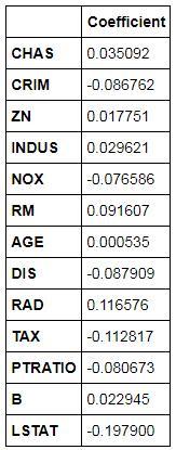
Calculating Accuracy: We can get the accuracy of this Ridge Regularized model by calculating the R2.

from sklearn import metrics
ridge_test_pred = pd.DataFrame({'actual':Y1_test,'predicted':Ridge.predict(X1_test)})
score_Ridge = metrics.r2_score(ridge_test_pred['actual'],ridge_test_pred['predicted'])
score_Ridge

By using a Ridge Regularized Linear Regression model, the accuracy comes out to be 71%.

Lasso

Lasso, unlike Ridge, forces the small coefficients to become zero. This way it technically removes certain variables from the analysis.

Initialise and Fit Linear Regression Model: We initialize the Regularized Linear Regression Model that uses the Lasso method of regularization and then fit it on the Train dataset. Here, we specify the value of alpha (=0.01) because the value of coefficients become zero as the value of alpha increases. By default, the value of alpha in Lasso is equal to 1, therefore, we reduced the value of alpha to 0.01.

Lasso = linear_model.Lasso(alpha=0.01)
Lasso.fit(X1_train,Y1_train)

Finding Coefficients: We can get the coefficients and unlike Ridge, here coefficients can/will become zero.

lasso_coef = pd.DataFrame(Lasso.coef_,X1_train.columns,columns=['Coefficient'])
lasso_coef

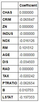
Calculating Accuracy: We can get the accuracy of this Lasso Regularized model by calculating the R2.

lasso_test_pred = pd.DataFrame({'actual':Y1_test,'predicted':Lasso.predict(X1_test)})
score_lasso = metrics.r2_score(lasso_test_pred['actual'],lasso_test_pred['predicted'])
score_lasso

The accuracy obtained by using the Lasso Regularized Model comes out to be 67%, while the accuracy that we got from Ridge was 71%. However, we can always select the features based on their coefficient value and adjust the value of alpha until we get the best possible results.

Feature Extraction

Here we will explore the most important method of Feature Extraction, which is Principal Component Analysis, and will use this method to reduce the features and use the output in modeling.

Importing Packages: We first import the important libraries.

import numpy as np
import pandas as pd
import matplotlib.pyplot as plt
%matplotlib inline
from sklearn.decomposition import PCA

Dataset: Here also we will be using the Boston Dataset. We will import a preprocessed dataset. This dataset has also been used in the Regression Problems using Python, where the preparation of this dataset has also been explored.

BosData = pd.read_excel('C:/Users/user/Desktop/R - Basic Stats/BosData.xls')
BosData.head()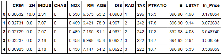

Removing Response Variable: As PCA works in an unsupervised learning setup, we will remove the dependent i.e. response variable from our dataset. Note that PCA only works on numeric variables, and that is why we create dummy variables for categorical variables. As here we have only one categorical variable, 'CHAS', which is a binary categorical variable, we don't require creating a dummy variable and can use all the independent variables for performing PCA.

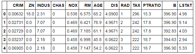
BosData2 = BosData[['CRIM', 'ZN', 'INDUS', 'CHAS', 'NOX', 'RM', 'AGE', 'DIS', 'RAD', 'TAX','PTRATIO', 'B', 'LSTAT']]
BosData2.head()

Scaling Features

Unlike R, there is no inbuilt PCA command option to scale the dataset. Therefore, we will have to first scale the dataset to perform PCA in Python.

from sklearn.preprocessing import StandardScaler
scale = StandardScaler()
scaled_data = scale.fit_transform(BosData2)
scaled_data

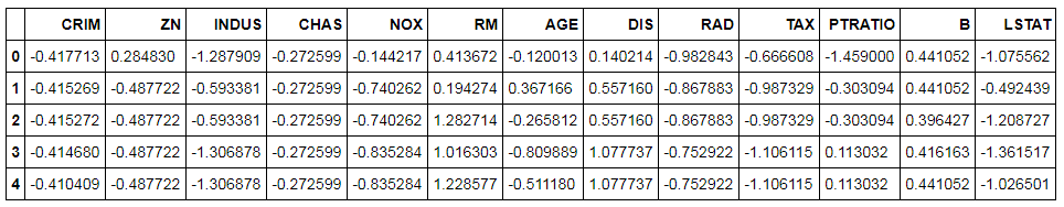
We can change the above output into a dataset.

scaled_data = pd.DataFrame(scaled_data,columns=BosData2.columns)
scaled_data.head()

Splitting the Dataset into Train and Test

It is important to note at this point that PCA should not be made to run on the entire dataset, as this would cause the dataset to leak, thus causing overfitting. Also, we should not perform PCA on train and test separately, as the level of variance will be different in both these datasets, which will cause the final vectors of these two datasets to have different directions. This is a Catch-22 situation and to get out of it we first divide the dataset into train and test and perform PCA on the train dataset and transform the test dataset using that PCA model (that was fitted on the train dataset). Below we use the sklearn package to split the data into train and test.

from sklearn.model_selection import train_test_split
Y = BosData['ln_Price']
X_train,X_test,Y_train,Y_test=train_test_split(scaled_data,Y,test_size=0.3,random_state=123)

Initialize and Fit PCA

We first initialize PCA for having 13 components (for 13 continuous variables in the dataset) and then we fit this model on the scaled features.

pca = PCA(n_components=13)
pca_model = pca.fit(X_train)

Generate PCA Loadings

We use the transform command, which transforms the scaled data to PCA loadings for each observation.

pca_train = pca_model.transform(X_train)
pca_train

Generate Loading Matrix

We now generate the principal components loading matrix by using the attribute components_ of the pca command for each variable.

Variable_Names = ['crim','zn','indus','chas','nox','rm','age','dis','rad','tax','ptratio','black','lstat']
Matrix = pd.DataFrame(pca_model.components_,columns=Variable_Names)
Matrix1 = np.transpose(Matrix)
Matrix1

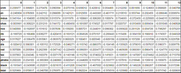
This Loading Matrix is like a correlation matrix. The variable having the highest correlation with the columns will be the first principal component. For example, the variable INDUS has the highest correlation with PC1, therefore, INDUS will be PC1. (The heading in the output is PC1, PC2 and so on. We will be renaming them in the upcoming steps.)

Variance Explained by Each Principal Component

As we saw above, we took the number of components for PCA equal to the number of variables in our dataset (which is 13 in our case). However, now with the following code, we will figure out the optimum value of the number of components to run PCA, i.e. reduce the number of components to be considered for the modeling algorithms and thus, in a way, reducing the number of features. In order to decide the number of Principal Components, we analyze the proportion of variance explained by each component. We use the explained_variance_ function for computing the variance explained by each Principal Component.

pca_model.explained_variance_

Ratio of Variance Explained by Each Component

We can now look at the proportion of variance explained by each PC.

var = pca_model.explained_variance_ratio_
var

From the output we find that PC1 explains 47% of the variance, PC2 explains 11%, and so on. We find that the first seven components explain approximately 90% of the variance (0.47818141 + 0.10745023 + 0.09150656 + 0.06383847 + 0.06069613 + 0.0528423 + 0.04414302 = 0.89865812).

PCA Chart

In the above step, we got the proportion of variance explained by each component, which we need to decide the number of components. We calculated that the first seven components explain most of the variance, however, for a more visual approach, we plot the explained variance on a line graph. Here we plot the ratio of variance explained by each component using a line graph. This PCA chart helps us to decide the number of principal components to be taken for the modeling algorithm.

cumulative_var = np.cumsum(np.round(var, decimals=4)*100)
plt.plot(cumulative_var,'k-o',markerfacecolor='None',markeredgecolor='k')
plt.title('Principal Component Analysis',fontsize=12)
plt.xlabel("Principal Component",fontsize=12)
plt.ylabel("Cumulative Proportion of Variance Explained",fontsize=12)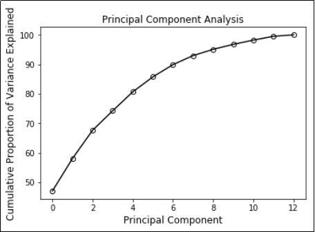

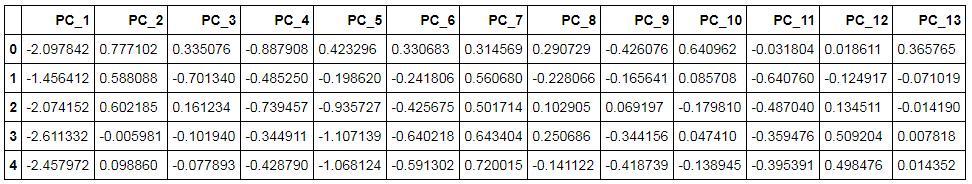
Renaming Columns

For our ease and convenience, we will rename the columns of the loading matrix that was generated for each observation using PCA. After renaming, we will select 7 principal components and make a data frame with the dependent variable and the 7 PCs.

pca_train = pd.DataFrame(pca_train,columns=['PC_' + str(i) for i in range(1,14)])
pca_train.head()

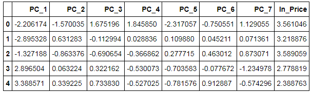
Concatenate Dependent Variable and Principal Components

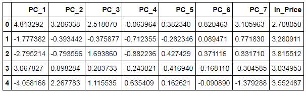
We now concatenate the dependent variable, i.e. ln_Price, with the principal components and take the first seven components for our analysis. First, we will reset the index for Y_train, as we need to concatenate datasets to make one whole train dataset. Then we will remove the index variable from the dataset and make a subset of the dataset having 7 PCs and the dependent variable.

Y_train1 = Y_train.reset_index()
pca_train1 = pd.concat([pca_train,Y_train1],axis=1)
pca_train2 = pca_train1.drop(columns='index')
pca_train3 = pca_train1[['PC_1', 'PC_2', 'PC_3', 'PC_4', 'PC_5', 'PC_6', 'PC_7','ln_Price']]

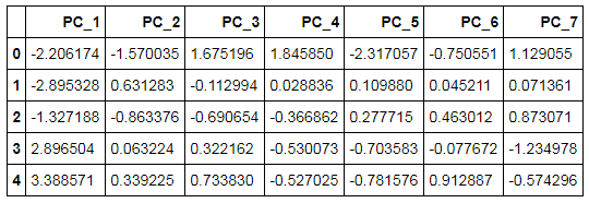
Creating Dataset having Principal Components

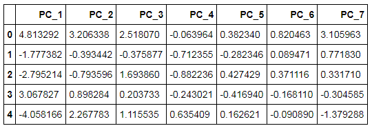
The above output forms the complete train dataset. As now we will be performing linear regression on this dataset, we are required to create a separate dataset having all the principal components, i.e. the independent features.

pca_train_X = pca_train3[['PC_1', 'PC_2', 'PC_3', 'PC_4', 'PC_5', 'PC_6', 'PC_7']]
pca_train_X.head()

Initializing and Fitting Linear Regression Model

We use linear_model from sklearn and initialize a Linear Regression Model.

linreg_model = linear_model.LinearRegression()
linreg_model.fit(pca_train_X,Y_train)

Transform Features of Test Dataset into Principal Components

As mentioned earlier, we will transform the features of the dataset into Principal Components using the PCA model created earlier.

pca_test = pca.transform(X_test)
pca_test

We now convert the above output into a dataset and add the dependent variable to it so that we can predict values using the above-created linear regression.

pca_test = pd.DataFrame(pca_test,columns=['PC_' + str(i) for i in range(1,14)])
Y_test1 = Y_test.reset_index()
pca_test1 = pd.concat([pca_test,Y_test1],axis=1)
pca_test1 = pca_test1.drop(columns='index')
pca_test2 = pca_test1[['PC_1', 'PC_2', 'PC_3', 'PC_4', 'PC_5', 'PC_6', 'PC_7','ln_Price']]
pca_test2.head()

Above we got the complete dataset. We now separate the Principal Components into a separate dataset.

pca_test_X = pca_test2[['PC_1', 'PC_2', 'PC_3', 'PC_4', 'PC_5', 'PC_6', 'PC_7']]
pca_test_X.head()

Prediction

We now predict the dependent variable of the test dataset using the linear regression model created earlier.

predict1 = linreg_model.predict(pca_test_X)

Results

We calculate the R-square to know the accuracy of our model.

from sklearn import metrics
metrics.r2_score(Y_test,predict1)

The accuracy comes out to be 63%.

Factor Analysis

Factor Analysis is a method which works in an unsupervised setup and forms groups of features by computing the relationship between the features. It is commonly used to reduce features and is explored in Factor Analysis under the theory section. We will now explore the application of Factor Analysis in Python.

Factor analysis can only be used to reduce continuous variables of the dataset. Therefore, we will be removing categorical variables. Again, like principal component analysis, this is an unsupervised learning algorithm, and hence we will be removing the dependent variable from our dataset.

Importing Preliminary Libraries: From factor_analyzer we will import FactorAnalyzer, which will come in handy for performing factor analysis.

from factor_analyzer import FactorAnalyzer

Dataset: We will be using the pre-processed Boston dataset that we have already normalized by creating a new variable ln_Price, which is the log of the dependent variable, i.e. Price.

Bos_train2 = pd.read_excel('C:/Users/user/Desktop/Data Sets/Linear Regression/Bos_train1.xls')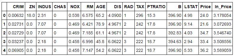

Removing the Dependent and Categorical Variables: As mentioned above, factor analysis works in an unsupervised setup only for the numerical variables, therefore, we will get rid of the categorical and the dependent variable.

Factor1 = Bos_train2[['CRIM', 'ZN', 'INDUS','NOX', 'RM', 'AGE', 'DIS', 'RAD', 'TAX','PTRATIO', 'B', 'LSTAT']]

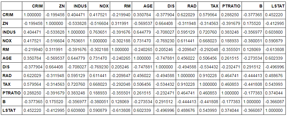
Creating Correlation Matrix for the above Dataset: To perform factor analysis we first create a correlation matrix using the above dataset. We can also manually analyse this matrix, as this will give us an idea of the variables that are highly correlated with each other.

corrm = Factor1.corr()
corrm

Finding Eigenvalues: We will now find the eigenvalues to decide the number of factors that will be sufficient for our modeling, i.e. deciding the number of variables we will use during modeling.

eigen_values = np.linalg.eigvals(corrm)
eigen_values_cumvar = (eigen_values/12).cumsum()
eigen_values_cumvar

Clearly, the four factors explain approximately 79% of the variance. Therefore, the number of factors will be equal to 4 in our case.

Using Factor Analyzer to Perform Factor Analysis: Now we will compute the factor loadings to group the variables based on their correlation values.

Factor_Analysis = FactorAnalyzer(n_factors=4, rotation='varimax', method='ml')
Factor_Analysis.fit(Factor1)

Here, we have used rotation equal to varimax to get maximum variance, and the method deployed for factor analysis is maximum likelihood. R and Python use the methods maximum likelihood or minres. However, other software such as SAS uses the method principal component analysis (PCA) to compute factor loadings.

We now compute the factor loadings.

loadings = pd.DataFrame(Factor_Analysis.loadings_, index=Factor1.columns)
loadings

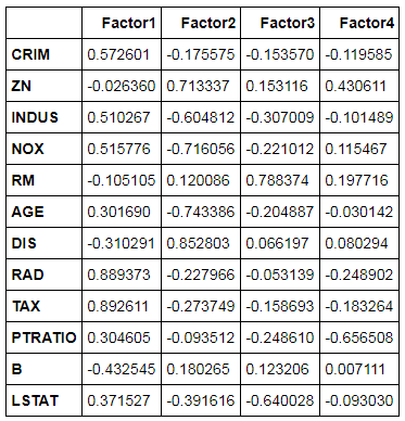
We now export the above output and sort it to find the 4 groups of features.

loadings.to_excel('C:/Users/user/Desktop/Data Sets/Linear Regression/python_FA.xls')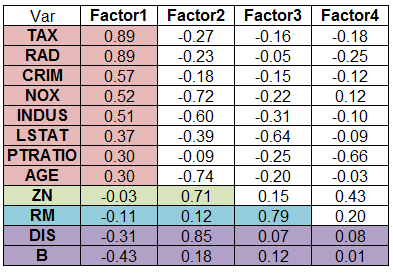

We can select variables for each of these groups, which will help us in decreasing the features and decreasing the chances of multicollinearity.

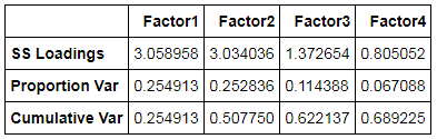
We can also compute the proportional variance and cumulative variance of the 4-factor solution.

Factor_Analysis.get_factor_variance()

In this blog post, we explored the application of the concepts mentioned in the Theory Section of Feature Engineering. Feature Engineering plays a crucial role in determining how well the learning algorithms will perform. It is important to Transform, Scale, Reduce and Construct features if it helps in increasing the quality of the data and makes the features more compatible with the various modeling algorithms. In the next section of application, all the concepts mentioned under the Theory Section of Modeling will be put to use using Python.